6.4 Working With Popular Packages

6.4.1 What is a package?

Up to this point in this book/course, we have really focused on using base R. By base, we simply mean the functions, data sets, and arguments that come pre-packaged with R. While this book has (hopefully) shown you just how much these basic functions can do, R can do so much more by relying on packages.

Packages are an integral part of R programming, and you have been using them throughout this book and class. A package is a contained set of arguments, operations, data, and/or other tools that don’t come with R. In general these are built by the vast community of R users and they cover tools from making beautiful maps in R to doing financial time-series analyses to downloading and analyzing hydrology data (see Vignettes). In fact, you have been using packages this whole time. For example, In order to knit a document using RMarkdown, you have to have the RMarkdown package installed.

On many (most?) projects, the most efficient way to complete whatever task you are doing is to spend at least some time checking out whether there is a package that makes it easier for you to do things like:

Download data from the internet
Perform statistical analyses
Plot data
Make maps
Add interactivity to your R code (like zoomable maps or plots)
And so much more!

6.4.2 How do I use packages?

There are always at least two steps to using any package.

Install the package using install.packages(). You only have to do this once.
Load the package using library(). You have to do this every time you want to use the capabilities of that package, but only once per Script or once per RMarkdown document.

Here is an example with an extremely common plotting package ggplot2 that has been mentioned in the course (and that you have probably already seen on the internet)

install.packages('ggplot2')

Now that we’ve installed the package, we can load it into R using library().

library('ggplot2')

Now that we have installed the package, we will need to learn how to use it. Where can we go to for help?

6.4.3 Finding and using package help.

All R packages installed with install.packages will come from the Comprehensive R Archive Network (“CRAN”). In order for you to work with them they have to have gone through a minimum overview, which ensures that they will at least have a minimum help page. So, for any package you want to read more about you can simply search for: CRAN <package name>. For ggplot2 this will lead you to this website. This site outlines many of the resources for using ggplot2, but they can be hard to find. The two most important places to look for help are the Reference manual and the URL.

The reference manual will outline every function that the package can perform and how to use the functions. ggplot2 is a big package so it has tons of functions, which is why you might not want to only use the PDF, which can be hard to navigate. Luckily they made a website that is more clear and has far more examples here.

6.4.4 Making Beautiful Plots with ggplot2

Our package is now loaded, and we have a manual for reference so let’s use it!

# Making up data for plotting
dat <- data.frame( response = c(1, 5, 10, 30, 100, 300),
                   driver = c(1, 2, 3, 4, 5, 6))

# Make a scatter plot with x and y 
ggplot(dat, aes(x = driver, y = response)) + 
  geom_point()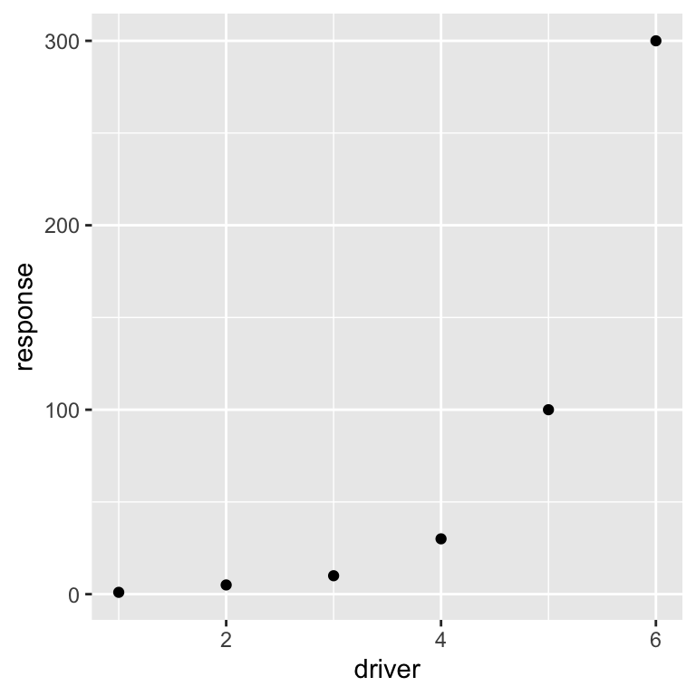

In the above command ggplot2 uses the data frame dat and the aesthetics (aes) argument to map which columns go where. In this case we want the driver variable to be on the x-axis and the response variable to be on the y-axis. Finally we want to use points to display this relationship between x and y (geom_point).

Note: ggplot2 connects a series of arguments using + operator. This is unique to ggplot, but it’s a helpful way to make complex plots by combining simpler pieces. This can be difficult to get used to, but can be very powerful once you get the hang of it.

Let’s add some lines to connect the points using the geom_line() command.

ggplot(dat, aes(x = driver, y = response)) + 
  geom_point() + 
  geom_line()  # Add lines to connect the points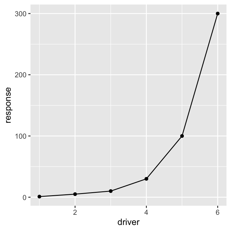

The geom prefix on the geom_point and geom_line functions stands for geometry. ggplot2 comes with many different types of geometries (see here ), and some folks have created their own packages to add even more options!

We can also change the way the lines and points look with arguments in the geom_point and geom_line functions:

ggplot(dat, aes(x = driver, y = response)) + 
  geom_point(color = "blue") +                     # Make the points blue
  geom_line(linetype = "dashed", color = "blue")   # Make the lines dashed and blue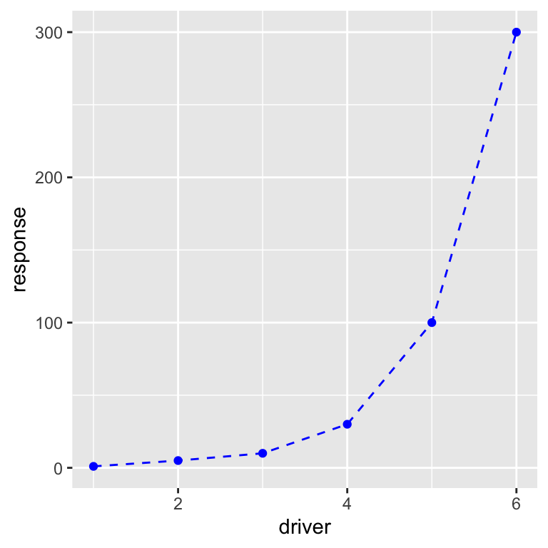

We can add a title and axis labels using the labs function:

ggplot(dat, aes(x = driver, y = response)) + 
  geom_point(color = "blue") + 
  geom_line(linetype = "dashed", color = "blue") + 
  labs(title = "Driver vs. Response",
       x = "Driver", y = "Response")   # Add labels to the plot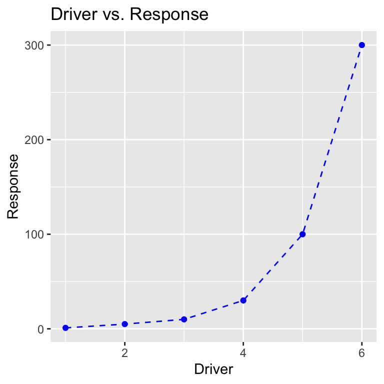

Finally, we can use one of the included ggplot2 themes to change how the plot looks, using the theme_set function:

theme_set(theme_minimal())   # Change the theme

ggplot(dat, aes(x = driver, y = response)) + 
  geom_point(color = "blue") + 
  geom_line(linetype = "dashed", color = "blue") + 
  labs(title = "Driver vs. Response",
       x = "Driver", y = "Response")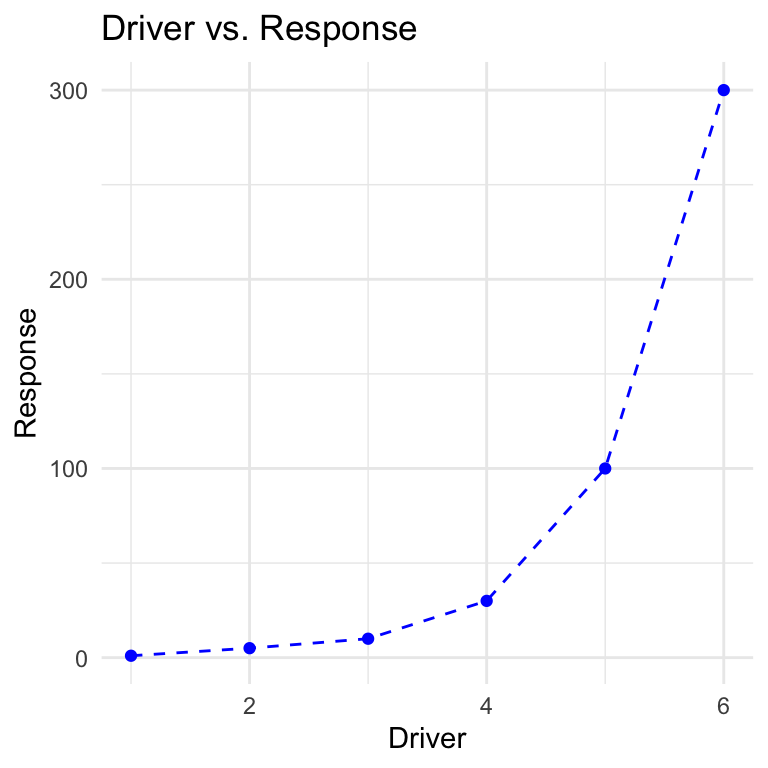

Here’s another example using the mtcars data frame, where we color the points based on their fuel economy (mpg) and annotate a few cars.

mtcars$car <- row.names(mtcars)  # Turn row names into a column so we can label with them

ggplot(mtcars, aes(x = hp, y = disp, color = mpg, label = car)) + 
  geom_point() + 
  geom_text(color = "black", hjust = 0,
            nudge_x = 5, alpha = 0.8, size = 2) +   # Annotate each car
  scale_color_viridis_c(option = "D") +             # Change color scale to use
  labs(title = "Motor Trend Car Comparison",
       x = "Horsepower", y = "Displacement", color = "MPG")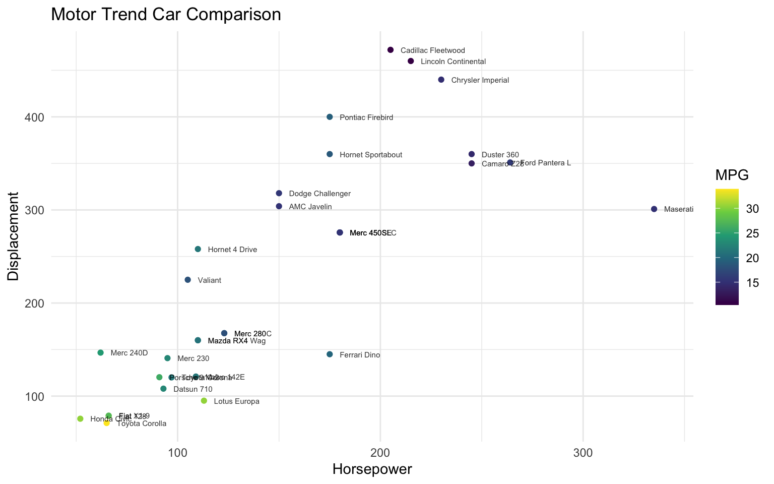

This is only scratching the surface of what ggplot2 can do, but hopefully this introduction is enough to hint at the possibilities. You can find many more examples at The R Graph Gallery.

(No need to turn this in) Create a plot of wt vs. mpg using the mtcars data frame using ggplot2. Make the points green.

6.4.5 Organizing Your Data With dplyr

As we saw, ggplot2 is a package intended to make nice looking visualizations in R easy. This is interesting, because R already has the capability to make plots, it’s just that ggplot2 is another way of making plots which many people think is more powerful. The same can be said about the next package we’ll discuss, dplyr (rhymes with “deep liar”), which is another way of manipulating data in R. We’ve spent a considerable amount of time on indexing, and you may have found the process somewhat confusing. Well, dplyr is another way of indexing data frames that many people find to be more intuitive. As always, you have to install dplyr if you haven’t already.

install.packages("dplyr")  # Install using quotes!

Then whenever you’d like to use the package, you have to load it:

library(dplyr)  # Load without using quotes!

Let’s look at some examples of base R indexing and compare that to how dplyr accomplishes the same task.

In base R, to select columns matching a certain condition, you create a logical vector and use it to index rows of the data frame.

index <- (mtcars$cyl == 4) & (mtcars$wt < 2)  # Select only columns with 4 cylinders and a weight under 2 tons
mtcars[index,]

In dplyr, the same thing can be accomplished with the filter function:

filter(mtcars, cyl == 4, wt < 2)  # Select only columns with 4 cylinders and a weight under 2 tons

This might already seem like an improvement, because it requires less code, but most people use the filter function differently than this. dplyr uses a pipe (which looks like this %>%) to structure arguments differently. Here’s how the same function looks with the pipe:

# Do the same filtering, but use the pipe, %>%
mtcars %>% filter(cyl == 4, wt < 2)

Basically, the pipe operator says “Take the thing on the left and use it as the first argument for the function on the right”. This may seem backwards at first, but it allows the chaining of multiple functions together in an order that reflects the order of computation that R will use (more on this after the next example). Recall that here’s how we select a column in base R:

mtcars[,"qsec"] # Select the qsec column

 [1] 16.46 17.02 18.61 19.44 17.02 20.22 15.84 20.00 22.90 18.30 18.90 17.40
[13] 17.60 18.00 17.98 17.82 17.42 19.47 18.52 19.90 20.01 16.87 17.30 15.41
[25] 17.05 18.90 16.70 16.90 14.50 15.50 14.60 18.60

And here’s how to do the same thing in dplyr:

mtcars %>% select(qsec)

Notice that dplyr has maintained the data frame structure, while indexing has not. We can get the same thing from indexing if we use the drop = F argument:

mtcars[,"qsec", drop = F]

The pipe works with the select function because the first argument of select is the data frame to select from, so the pipe says “Use mtcars as the first argument of the select function”. Here’s how we would do the filtering and selection at the same time in dplyr:

mtcars %>% 
  filter(cyl == 4, wt < 2) %>%
  select(qsec)

Since the result of the filter function is a data frame (which is why it printed in the result in the example above!), that data frame can be piped into the select function. This easy chaining of arguments is one reason why people love to work with tidyverse packages.

The pipe operator is one of the most common elements of the tidyverse group of packages. One of the tidyverse packages called magrittr even uses the pipe operator as its official logo, with the slogan “Ceci n’est pas un pipe”, a reference to this famous work of art.

dplyr can also summarize columns in different groups similarly to the tapply function. Here’s an example of tapply:

# Find the mean mpg for different numbers of cylinders:
tapply(mtcars$mpg, mtcars$cyl, mean)

       4        6        8 
26.66364 19.74286 15.10000

In dplyr this is accomplished with the group_by and summarize functions:

mtcars %>% 
  group_by(cyl) %>%
  summarize(ave_mpg = mean(mpg))

With only a few functions, we can now start to chain together quite complex operations in a human readable way:

mtcars %>%
  filter(wt > 2) %>%       # Filter out cars below 2 tons
  group_by(cyl, gear) %>%  # Group by number of cylinders and number of gears
  summarize(n = n(),              # Compute number of cars in each group
            ave_mpg = mean(mpg),  # Compute average mpg
            sd_mpg = sd(mpg))     # Compute standard deviation of mpg

`summarise()` has grouped output by 'cyl'. You can override using the `.groups`
argument.

Again, this is only a teaser of the capabilities of dplyr, but the hope is that if/when you encounter dplyr in the future, you will at least have an introduction to some of the basic concepts.

6.4.6 Working With Character Strings with stringr

stringr is another tidyverse package that provides functions for easily working with character strings.

# install.packages("stringr")  # Install if you haven't before 
library(stringr)

To show some of the capabilities of the stringr package, we’ll read in “Pride and Prejudice” which is available on Project Gutenberg here.

lines <- readLines(file("data_raw/pride_and_prejudice.txt", "rt"))
length(lines)  # The book is now a long character vector

[1] 14594

The first thing we’ll do is convert the text into “UTF-8” formatting using stringr’s str_conv function:

lines <- str_conv(lines, "UTF-8")

Right now, each element of lines is just a single line from the original text file. Let’s collapse all the elements into a single character string:

book <- str_c(lines, collapse=" ")
nchar(book)

[1] 775739

Now we can split the book in a more sensible way. Let’s split the string at the end of each sentence using the strsplit function (this is a base R function, actually).

sent <- strsplit(book, "(?<=[[:punct:]])\\s(?=[A-Z])", perl = T)  # Split by end of sentences
sent <- unlist(sent)  # Convert list to character vector
length(sent)

[1] 5175

The strsplit function above used something called a regular expression to identify patterns that indicate the end of a sentence. Regular expressions are commonly used in programming, and can be confusing when first encountered. This is okay! You might want to take a look at this resource if you want more info on regular expressions in R.

The sent vector now contains sentences as elements. Let’s look at an arbitrary sentence:

sent[300]

[1] "I should think she had       as good a chance of happiness as if she were to be studying his       character for a twelvemonth."

We notice that there are some extra spaces in the sentence, which probably result from the formatting of the original text file. Ignoring that for now, we can find all sentences containing the word “Jane”:

has_jane <- str_detect(sent, "Jane") # Returns logical vector 
sum(has_jane)

[1] 265

We see there are 265 sentences with the string “Jane” in them. Let’s look at some of them:

jane_sent <- sent[has_jane]
jane_sent[100:105]

[1] "She could think of nothing       else; and yet whether Bingley’s regard had really died away, or       were suppressed by his friends’ interference; whether he had been       aware of Jane’s attachment, or whether it had escaped his       observation; whatever were the case, though her opinion of him       must be materially affected by the difference, her sister’s       situation remained the same, her peace equally wounded.        A day or two passed before Jane had courage to speak of her       feelings to Elizabeth; but at last, on Mrs."
[2] "It cannot last long.       He will be forgot, and we shall all be as we were before.”        Elizabeth looked at her sister with incredulous solicitude, but       said nothing.        “You doubt me,” cried Jane, slightly colouring; “indeed, you have       no reason."                                                                                                                                                                                                                                                                                        
[3] "A little time, therefore—I shall certainly try to       get the better.”        With a stronger voice she soon added, “I have this comfort       immediately, that it has not been more than an error of fancy on       my side, and that it has done no harm to anyone but myself.”        “My dear Jane!” exclaimed Elizabeth, “you are too good."                                                                                                                                                                                                               
[4] "My       dear Jane,"                                                                                                                                                                                                                                                                                                                                                                                                                                                                                                                                               
[5] "You shall not, for the sake of one individual, change the       meaning of principle and integrity, nor endeavour to persuade       yourself or me, that selfishness is prudence, and insensibility       of danger security for happiness.”        “I must think your language too strong in speaking of both,”       replied Jane; “and I hope you will be convinced of it by seeing       them happy together."                                                                                                                                                 
[6] "They may wish many things besides       his happiness; they may wish his increase of wealth and       consequence; they may wish him to marry a girl who has all the       importance of money, great connections, and pride.”        “Beyond a doubt, they do wish him to choose Miss Darcy,” replied       Jane; “but this may be from better feelings than you are       supposing."

We can also count the number of occurrences of a string in the book using the str_count function:

str_count(book, "pride")

[1] 46

str_count(book, "prejudice")

[1] 8

To see more capability of the stringr package, you can check out this cheat sheet.

Any feedback for this section? Click here