5.3 Summary Statistics
Reading and writing data is useful, but the power of R is doing interesting things with the data!
Let’s perform a few operations with the Olympic athletes data to demonstrate some important functions for data analysis.
As we’ve seen, the summary function automatically performs some summary statistics on each column of a data frame.
Let’s see how to produce these and other results manually.
5.3.1 Quantitative Variables
To showcase the functions R provides to summarize quantitative variables, we’ll look at the Age column of our data frame, which is stored as an integer vector in R.
What other R data types might be used to store quantitative data?
However, Age contains NA values, as we know from running the following function:
[1] 183is.na function returns a logical array which is true whenever the Age column is NA. So why does the sum function produce the number of NA’s?
As a cleaning step, we must first remove the NA values:
age <- athletes$Age       # Assign the Ages column to a variable
age <- age[!is.na(age)]   # Extract only the elements which are not NA (more on this when we discuss advanced indexing)
This type of “data cleaning” is a very common first step when performing data analysis. You will get more opportunities to clean data later in the course.
Here are some functions R provides to summarize quantitative variables.
age_min <- min(age)     # Find the minimum age
age_med <- median(age)  # Find the median age
age_max <- max(age)     # Find the maximum age
age_mean <- mean(age)   # Find the average age
age_sd <- sd(age)       # Find the standard deviation of age
age_var <- var(age)     # Find the variance of age
Let’s put all these results in a named list. In the following code, read the comments carefully to understand how the code is being organized onto multiple lines.
# Create a list containing all the stats
age_stats <- list(  # R knows that this command continues until a closed parenthesis
  min = age_min,
  median = age_med,
  max = age_max,
  mean = age_mean,
  sd = age_sd,
  var = age_var
)  # This could all go on one line, but it looks more organized this way.
age_stats
$min
[1] 12
$median
[1] 25
$max
[1] 74
$mean
[1] 25.65373
$sd
[1] 6.495693
$var
[1] 42.19402weight_stats with the mean, median, and standard deviation of the Weight column.
If you get NA values for the statistics, you should include the na.rm=T argument like so: mean(weight, na.rm=T), to remove the NA values before computing the statistics.
Visualization will be discussed more later, but we’ll show one plot now, to show how multiple summary statistics can be shown at the same time.
hist(age, breaks = 50)
abline(v = age_mean, col = "blue", lty = 2, lwd = 3)
abline(v = age_med, col = "red", lty = 2, lwd = 3)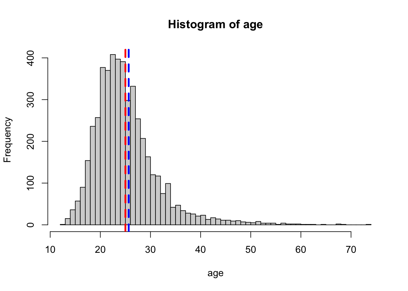 It looks like the distribution of
 Age is right skewed, consistent with the fact that the mean is greater than the median.
Of course, having more than one quantitative variable allows us to compare them against each other. Here’s how to compute the covariance between two quantitative variables:
[1] 6.483675
The argument use=“complete.obs” is one way to deal with
NA values in the cov function. This makes R
remove any observations which are NA in either the first or second
variable. There are other ways as well, which you can check using the
help function: ?cov.
You can also compute the correlation between two variables like so:
[1] 0.1104457Using the cov or cor functions on an entire data frame or matrix will produce a correlation matrix of the columns.
Here’s an example with the mtcars data frame:
            mpg        cyl       disp         hp        drat         wt
mpg   1.0000000 -0.8521620 -0.8475514 -0.7761684  0.68117191 -0.8676594
cyl  -0.8521620  1.0000000  0.9020329  0.8324475 -0.69993811  0.7824958
disp -0.8475514  0.9020329  1.0000000  0.7909486 -0.71021393  0.8879799
hp   -0.7761684  0.8324475  0.7909486  1.0000000 -0.44875912  0.6587479
drat  0.6811719 -0.6999381 -0.7102139 -0.4487591  1.00000000 -0.7124406
wt   -0.8676594  0.7824958  0.8879799  0.6587479 -0.71244065  1.0000000
qsec  0.4186840 -0.5912421 -0.4336979 -0.7082234  0.09120476 -0.1747159
vs    0.6640389 -0.8108118 -0.7104159 -0.7230967  0.44027846 -0.5549157
am    0.5998324 -0.5226070 -0.5912270 -0.2432043  0.71271113 -0.6924953
gear  0.4802848 -0.4926866 -0.5555692 -0.1257043  0.69961013 -0.5832870
carb -0.5509251  0.5269883  0.3949769  0.7498125 -0.09078980  0.4276059
            qsec         vs          am       gear        carb
mpg   0.41868403  0.6640389  0.59983243  0.4802848 -0.55092507
cyl  -0.59124207 -0.8108118 -0.52260705 -0.4926866  0.52698829
disp -0.43369788 -0.7104159 -0.59122704 -0.5555692  0.39497686
hp   -0.70822339 -0.7230967 -0.24320426 -0.1257043  0.74981247
drat  0.09120476  0.4402785  0.71271113  0.6996101 -0.09078980
wt   -0.17471588 -0.5549157 -0.69249526 -0.5832870  0.42760594
qsec  1.00000000  0.7445354 -0.22986086 -0.2126822 -0.65624923
vs    0.74453544  1.0000000  0.16834512  0.2060233 -0.56960714
am   -0.22986086  0.1683451  1.00000000  0.7940588  0.05753435
gear -0.21268223  0.2060233  0.79405876  1.0000000  0.27407284
carb -0.65624923 -0.5696071  0.05753435  0.2740728  1.00000000
However, this only works if all columns of the data frame (or matrix) are numeric. Here’s what happens if we try the same thing on the athletes data:
Error in cor(athletes): 'x' must be numeric
5.3.2 Categorical Variables
To showcase the functions R provides for categorical variables, we’ll look, at the Sport column, which is stored as a character vector in R.
What other R data types might be used to store categorical data?
Are there any NA values in this column?
[1] 0It turns out the answer is no, so there’s no need to remove anything. In a character vector like this, we expect there to be many duplicated values. We can see a list of all the unique values with the following:
 [1] "Hockey"                    "Wrestling"
 [3] "Swimming"                  "Basketball"
 [5] "Biathlon"                  "Speed Skating"
 [7] "Fencing"                   "Weightlifting"
 [9] "Equestrianism"             "Archery"
[11] "Cross Country Skiing"      "Gymnastics"
[13] "Tennis"                    "Athletics"
[15] "Cycling"                   "Bobsleigh"
[17] "Shooting"                  "Sailing"
[19] "Alpine Skiing"             "Art Competitions"
[21] "Canoeing"                  "Football"
[23] "Rowing"                    "Figure Skating"
[25] "Nordic Combined"           "Judo"
[27] "Short Track Speed Skating" "Water Polo"
[29] "Snowboarding"              "Taekwondo"
[31] "Diving"                    "Handball"
[33] "Softball"                  "Boxing"
[35] "Tug-Of-War"                "Ski Jumping"
[37] "Table Tennis"              "Ice Hockey"
[39] "Modern Pentathlon"         "Golf"
[41] "Baseball"                  "Volleyball"
[43] "Luge"                      "Badminton"
[45] "Trampolining"              "Curling"
[47] "Beach Volleyball"          "Polo"
[49] "Rugby Sevens"              "Synchronized Swimming"
[51] "Triathlon"                 "Skeleton"
[53] "Freestyle Skiing"          "Military Ski Patrol"
[55] "Lacrosse"                  "Rhythmic Gymnastics"
[57] "Rugby"
Using the numbers in brackets to the left as our guide, we can see that there are 57 unique values, but this can also be determined by running:
[1] 57It would be nice to see how many times each entry occurs in the data set.
This is what the table function does:
sport
            Alpine Skiing                   Archery          Art Competitions
                      148                        41                        64
                Athletics                 Badminton                  Baseball
                      728                        32                        19
               Basketball          Beach Volleyball                  Biathlon
                       98                        18                       100
                Bobsleigh                    Boxing                  Canoeing
                       53                       121                       112
     Cross Country Skiing                   Curling                   Cycling
                      174                         8                       205
                   Diving             Equestrianism                   Fencing
                       56                       121                       184
           Figure Skating                  Football          Freestyle Skiing
                       44                       138                         9
                     Golf                Gymnastics                  Handball
                        5                       498                        61
                   Hockey                Ice Hockey                      Judo
                      101                        83                        76
                 Lacrosse                      Luge       Military Ski Patrol
                        1                        25                         2
        Modern Pentathlon           Nordic Combined                      Polo
                       37                        25                         4
      Rhythmic Gymnastics                    Rowing                     Rugby
                        9                       190                         4
             Rugby Sevens                   Sailing                  Shooting
                        6                       126                       218
Short Track Speed Skating                  Skeleton               Ski Jumping
                       23                         4                        45
             Snowboarding                  Softball             Speed Skating
                       19                        10                       104
                 Swimming     Synchronized Swimming              Table Tennis
                      399                         9                        36
                Taekwondo                    Tennis              Trampolining
                       10                        45                         4
                Triathlon                Tug-Of-War                Volleyball
                        6                         5                        50
               Water Polo             Weightlifting                 Wrestling
                       79                        85                       123
Let’s save this table to a list as before:
# Assign summary statistics to variables
sport_n_unique <- length(unique(sport))
sport_counts <- table(sport)

# Combine them into a list
sport_stats <- list(
  number_unique = sport_n_unique,
  counts = sport_counts
)
Again, a visualization may be useful here:
par(mar = c(5, 15, 4, 2) + 0.1)  # Command to make the labels fit
barplot(table(sport), horiz = T, las = 2)  # Bar plot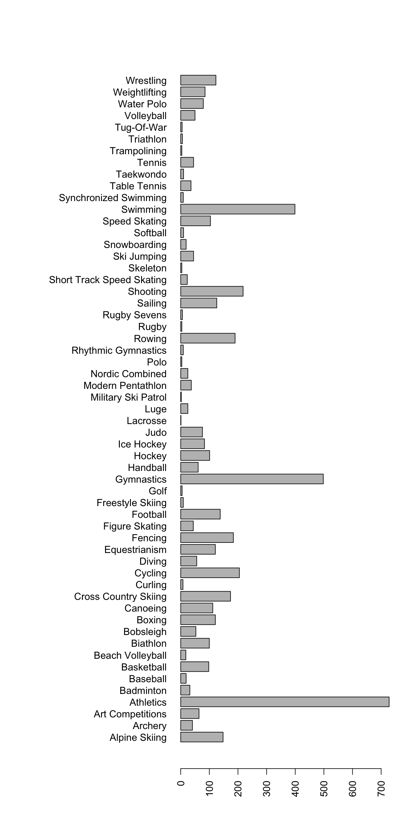
So we see that in our data set, athletics, swimming, and gymnastics have the most athletes (remember, each row is an athlete).
season_stats with a table of counts for the Season variable.
Height, Weight, and Sex variables? Can you give an example of what might happen? What other variables may be impacted? What R code would you write to determine if an athlete occurred multiple times in the data frame?
5.3.3 Saving an RData file
Finally, we may want to save these results for use in R later. First, we’ll create a new list to put our two stats list in (remember, we can have lists inside of other lists!).
Remember that the names function retrieves the column names for a data frame? It also retrieves the names of a list (after all, a data frame is just a fancy list, right?)!
The following commands may be useful for remembering what the contents of our stats list:
names(athlete_stats)names(athlete_stats$age)names(athlete_stats$sport)
To save these results, we can use the saveRDS function:
Later, we can use the following command to load the RDS file back into R:
rm(athlete_stats)  # Remove athlete stats to prove we are loading it from the hard drive

athlete_stats <- readRDS("data_clean/athlete_stats.rds")  # Load the RDS file and name it athlete_stats

athlete_stats$age  # Show that we have loaded the data by printing the age stats
$min
[1] 12
$median
[1] 25
$max
[1] 74
$mean
[1] 25.65373
$sd
[1] 6.495693
$var
[1] 42.19402The RDS format works for any R Object, not just lists, so it can be used for vectors, matrices, factors, and even functions.
Any feedback for this section? Click here