5.7 Vignettes
In this section, you’ll gain more experience working with data by following along with some more data analysis examples.
5.7.1 Flood analysis example
In this example we will learn how to analyze flood data to better understand the history of flooding in the last ten years in the Cache La Poudre river which runs through Fort Collins. This vignette will help you learn three key ideas:
Data can be read into R directly from online data services using
packageswhich you will learn about later in this book.We can use this ‘live’ data to understand both past and present river conditions in the river.
We can use R to look at changes over time in river flow and water height.
5.7.1.1 Map
The river monitoring location for the Cache La Poudre River is right at Lincoln Bridge near Odell Brewing.
5.7.1.2 Installing and using packages
In order to download river flow and height data we will first need to load a
package called dataRetrieval this is a package run by the United States
Geological Survey (USGS) and it provides access to data from over 8000
river monitoring
stations in the United States and millions of water quantity and quality
records. You can learn more about the data from the USGS here. To use packages we first have
to install them using the command install.packages and then load them
using the command library.
5.7.1.3 Downloading the data
Once we have loaded the package we can use
the special functions that it brings to the table. In this case, dataRetrival
provides a function called readNWISdv which can download daily data
(or daily values, hence readNWISdv) for specific
monitoring locations. But how do we use this function?
Try ?readNWISdv to get more details.
So the readNWISdv command requires a few key arguments. First
siteNumbers, these are simply the site identifiers that the USGS uses
to track different monitoring stations and in our case that number for the
Cache La Poudre is 06752260, which you can find here.
The second argument is the parameterCd which
is a cryptic code that indicates what kind of data you want to download. In
this case we want to download river flow data. River
flow tells us how much water is moving past a given point and is correlated
with the height of the river water. This code is 00060 for discharge which means
river flow.
Lastly we need to tell the readNWISdv command the time period for which we want
data which is startDate which we will set to 2010,
and endDate which we will set to the current day using the command
Sys.Date(). These arguments should be in the
YYYY-MM-DD format. With all this knowledge of how the command works, we can
finally download some data, directly into R!
poudre <- readNWISdv(siteNumbers = '06752260',
                     parameterCd = c('00060'),
                     startDate = '2010-10-01',
                     endDate = Sys.Date())
GET: https://waterservices.usgs.gov/nwis/dv/?site=06752260&format=waterml,1.1&ParameterCd=00060&StatCd=00003&startDT=2010-10-01&endDT=2025-02-285.7.1.4 Explore the data structure
Now that we have our dataframe called poudre, we can explore the properties
of this data frame using commands we have already learned. First let’s
see what the structure of the data is using the head command, which
will print the first 6 rows of data.
It looks like we have a dataframe that is 5 columns wide with columns agency_cd which is just the USGS, site_no which is just the site id we already told it. Since
we only asked for data from one site, we don’t really need this column. A Date
column which tells us… the date! There are two more columns that are kind of weird which
are labeled X_00060_00003 which is the column that actually has values of
river flow in Cubic Feet Per Second (cfs), or the amount of water that is flowing
by a location per second in Cubic Feet volume units (1 cubic foot ~ 7.5 gallons).
Finally X_00060_00003_cd tells us something about the quality of the data. For now
we will ignore this final column, but if you were doing an analysis of this data
for a project, you would want to investigate what codes are acceptable for
high quality analyses. To make working with this data a little easier let’s
rename and remove some of our columns in a new, simpler dataframe.
5.7.1.5 Explore the data
Now that we have cleaned up our data frame a little, let’s explore the data.
First we can use the summary function to just quickly look at the variables we have.
      Date                q_cfs
 Min.   :2010-10-01   Min.   :   1.31
 1st Qu.:2014-05-08   1st Qu.:  22.85
 Median :2017-12-14   Median :  59.80
 Mean   :2017-12-14   Mean   : 215.15
 3rd Qu.:2021-07-22   3rd Qu.: 140.00
 Max.   :2025-02-27   Max.   :7150.00
                      NA's   :25
It looks like we have data from 2010 to 2025-02-28 and a range in river flow (q_cfs) from 2.6 cfs all the way up to 7150 cfs. If you’re a hydrologist, hopefully these flow numbers look right, but another way to check to make sure is to simply plot the data as we do below.
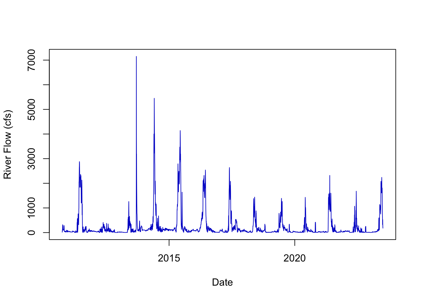
The above plot is called a “hydrograph” or a plot of how river flow has changed over time. In the Cache La Poudre, what might explain the peaks and valleys of the data? What controls river flow in Colorado rivers?
5.7.1.6 Analyze the data
Now that we’ve plotted the data we can see some interesting patterns that we
might want to explore. For example, how has the average flow changed in the last
ten years. To analyze this, we need to use the concept of a Water Year. Simply
put, a water year is a way to analyze yearly variation in flow, which doesn’t
map well to a calendar year. Water years in the USA are typically from October 1
to September 30th. Luckily for us, the dataRetrieval package has a function
that calculates water year for us. It’s simply called addWaterYear.
To look at variation per year we can use the function tapply which can take the mean, max or any summary
function of groups of data (more on this in the next chapter, but you can type ?tapply for more info).
In this case, we want to look at the mean river flow for each water year.
Now to use tapply we use the following code
Now let’s plot the data, where the values (y) are the annual average flow and the years (x) are the names of the annual vector from the tapply function.
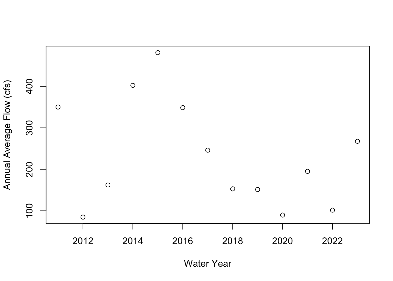
Has annual mean river flow declined over the past ten years? What about the last 6?
Any feedback for this section? Click here