5.1 Scraping in the Wild
In Chapter 2, we introduced the idea of rectangular data vs. non-rectangular data, providing examples for each and demonstrating the process of rectangularization. We outlined how to use a web-API before introducing the concept of web scraping by illustrating the language of the web: HTML. Since webpages can be complicated, scraping can be complicated. In this chapter, we will leverage the Selector Gadget and our knowledge of HTML elements to scrape data from various sources. It is our belief that the only way to teach web scraping is through examples. Each example will become slightly more difficult than the previous.
5.1.1 Lessons Learned from Scraping
Scraping is a necessary evil that requires patience. While some tasks may prove easy, you will quickly find others seem insurmountable. In this section, we will outline a few tips to help you become a web scraper.
Brainstorm! Before jumping into your scraping project, ask yourself what data do I need and where can I find it? If you discover you need data from various sources, what is the unique identifier, the link which ties these data together? Taking the time to explore different websites can save you a vast amount of time in the long run. As a general rule, simplistic looking websites are generally easier to scrape and often contain the same information as more complicated websites with several bells and whistles.
Start small! Sometimes a scraping task can feel daunting, but it is important to view your project as a war, splitting it up into small battles. If you are interested in the racial demographics of each of the United States, consider how you can first scrape this information for one state. In this process, don’t forget tip 1!
Hyperlinks are your friend! They can lead to websites with more detailed information or serve as the unique identifier you need between different data sources. Sometimes you won’t even need to scrape the hyperlinks to navigate between webpages, making minor adjustments to the web address will sometimes do.
Data is everywhere! Text color, font, or highlighting may serve as valuable data that you need. If these features exist on the webpage, then they exist within the HTML code which generated the document. Sometimes these features are well hidden or even inaccessible, leading to the last and final tip.
Ready your search engine! Just like coding in
Ris an art, web developing is an art. When asking distinct developers to create the same website with the same functionality, the final result may be similar but the underlying HTML code could be drastically different. Why does this matter? You will run into an issue that hasn’t been addressed in this text. Thankfully, if you’ve run into an issue, someone else probably has too. We cannot recommend websites like Stack Overflow enough.
5.1.2 Scraping NFL Data
In Chapter 2, we gathered some betting data pertaining to the NFL through a web-API. We may wish to supplement these betting data with data pertaining to NFL teams, players, or even playing conditions. As we progress through this sub-section, examples will become increasingly problematic or troublesome. The goal in this subsection is to introduce you to scraping by heeding the advice given in the Chapter 5.1.1.
Following our own advice, let’s brainstorm. When you think of NFL data, you probably think of NFL.com or ESPN. After further digging, we will explore Pro Football Reference, a reliable archive for football statistics (with a reasonably simple webpage). This is an exhaustive source which boasts team statistics, player statistics, and playing conditions for various seasons. Let’s now start small by focusing on team statistics, but further, let’s limit our scope to the 2020 Denver Broncos. Notice, there are hyperlinks for each player documented in any of the categories, as well hyperlinks for each game’s boxscore where there is information about playing conditions and outcomes. Hence, we have a common thread between team statistics, players, and boxscores. If, for example, we chose to scrape team statistics from one website and player statistics from another website, we may have to worry about a unique identifier (being team) if the websites have different naming conventions.
5.1.2.1 HTML Tables: Team Statistics
We’ll start with the team statistics for the 2020 Denver Broncos which can be found in a table entitled ‘Team Stats and Rankings’. We’ll need to figure in which element or node the table lives within the underlying HTML. To do this, we will utilize the CSS selector gadget. If we highlight over and click the table with the selector gadget, we will see that the desired table lives in an element called ‘#team_stats’.
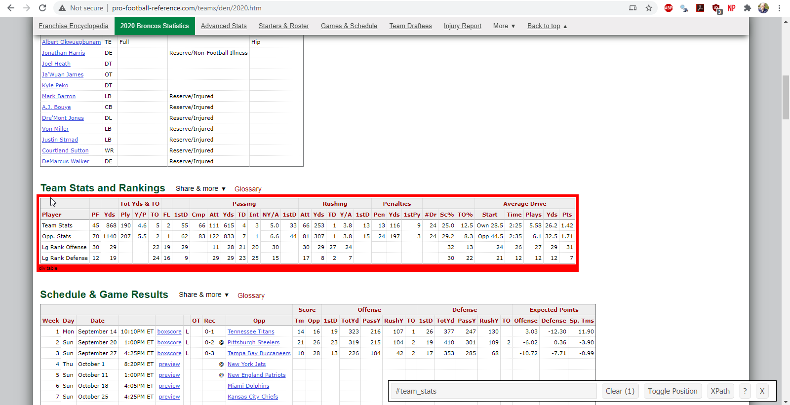
Figure 5.1: finding the team statistics element using the selector gadget
Alternatively, we could view the page source and search for the table name. I’ve highlighted the information identified by the selector gadget with the cursor.
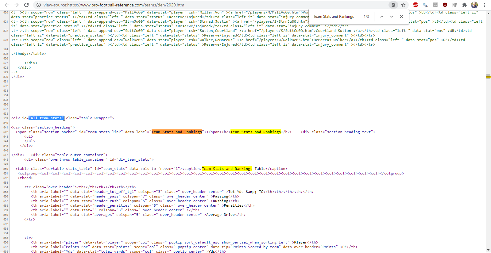
Figure 5.2: finding the team statistics element using the page source
While the selector gadget is always a great first option, it is not always reliable. There are instances when the selector gadget identifies a node that is hidden or inaccessible without JavaScript. In these situations, it is best view the page source directly for more guidance on how to proceed. Practice with both the selector gadget and the page source.
Once we have found the name of the element containing the desired data, we can utilize the rvest package to scrape the table. The general process for scraping an HTML table is
- Read the HTML identified by the web address.
- Isolate the node containing the data we desire.
- Parse the HTML table.
- Take a look at the data to ensure the columns are appropriate labels.
library(rvest)
library(janitor)

pfr_url <- "https://www.pro-football-reference.com"
broncos_url <- str_c(pfr_url, '/teams/den/2020.htm')

broncos_url %>%
  # read the HTML
  read_html(.) %>%
  # isolate the node containing the HTML table
  html_node(., css = '#team_conversions') %>%
  # parse the html table
  html_table(.) %>%
  # make the first row of the table column headers and clean up column names
  row_to_names(., row_number = 1) %>%
  clean_names()
While these data need cleaning up before they can be used in practice, we will defer these responsibilities to Chapter 3.
In the next subsection, we will take a deeper dive into scraping HTML tables using information attained from attribute values, a common occurrence in web scraping. Take this time to scrape the ‘Team Conversions’ table on your own.
Any feedback for this section? Click here
5.1.2.3 Attributes: Player Statistics by Game
Suppose now that we wish to scrape the same player statistics, but rather than get the aggregated total, we want the players’ statistics by game. Within the Rushing and Receiving table scraped in the previous example, there are hyperlinks for each player. When you click on this hyperlink, you will find the player’s statistics for each game played. These are the data we desire. We want rushing and receiving statistics for each player on each team for a variety of years. Using the lessons learned in Chapter 5.1.1, we have brainstormed the problem and have a road map to the solution. We will first scrape the hyperlink attribute to get the web address associated with each player for a given team. Within each of these web addresses, we will scrape the game by game statistics before iterating over each team in the NFL. After this, we can repeat the procedure for a variety of years. This is, of course, a big job, so let’s scale down the problem to one player: Melvin Gordon III, running back. To do this, we will:
- Get the web addresses associated with each player in the Rushing and Receiving table, before isolating the address associated with Melvin Gordon’s rushing and receiving statistics.
- Read the HTML identified by the web address.
- Isolate the node containing the data we desire.
- Parse the HTML table.
- Take a look at the data to ensure the columns are appropriate labels.
Let’s figure out where the hyperlinks exist within the HTML code. To do this, I will look at the page source and search for Melvin Gordon. We find that the web address corresponding to his game by game player statistics exist in the hidden HTML table that we scraped in the previous example. In particular, they are the href attribute to a node entitled a which is embedded within the hidden HTML table. Phew. Let’s consider how we can scrape these web addresses step by step:
1.1 Isolate the hidden HTML table, similar to the previous example.
1.2 Isolate nodes with tag a.
1.3 Extract the href attribute from these nodes.
Steps 1.1 and 1.2 should be familiar from previous examples, but step 1.3 requires a new function within rvest called html_attr. Let’s see how to do this in R.
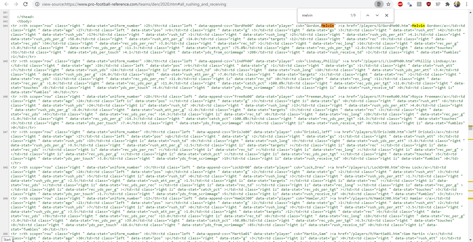
Figure 5.3: finding the element containing the web address cooresponding to Melvin Gordon III game by game player statistics using the page source
player_urls <- broncos_url %>%
  read_html() %>%
  html_node(., css = '#all_rushing_and_receiving') %>%
  html_nodes(., xpath = 'comment()') %>%
  html_text() %>%
  read_html() %>%
  html_nodes(., 'table') %>%
  html_nodes(., 'a') %>%
  html_attr(., 'href') %>%
  str_c(pfr_url, .)
player_urls
[1] "https://www.pro-football-reference.com/players/G/GordMe00.htm"
[2] "https://www.pro-football-reference.com/players/L/LindPh00.htm"
[3] "https://www.pro-football-reference.com/players/L/LockDr00.htm"
[4] "https://www.pro-football-reference.com/players/F/FreeRo00.htm"
[5] "https://www.pro-football-reference.com/players/H/HamlKJ00.htm"
[6] "https://www.pro-football-reference.com/players/D/DrisJe00.htm"
[7] "https://www.pro-football-reference.com/players/R/RypiBr00.htm"
[8] "https://www.pro-football-reference.com/players/B/BellLe02.htm"
[9] "https://www.pro-football-reference.com/players/S/SpenDi00.htm"
[10] "https://www.pro-football-reference.com/players/H/HintKe00.htm"
[11] "https://www.pro-football-reference.com/players/M/MartSa01.htm"
[12] "https://www.pro-football-reference.com/players/F/FantNo00.htm"
[13] "https://www.pro-football-reference.com/players/J/JeudJe00.htm"
[14] "https://www.pro-football-reference.com/players/P/PatrTi00.htm"
[15] "https://www.pro-football-reference.com/players/H/HamiDa01.htm"
[16] "https://www.pro-football-reference.com/players/V/VannNi00.htm"
[17] "https://www.pro-football-reference.com/players/O/OkwuAl00.htm"
[18] "https://www.pro-football-reference.com/players/F/FumaTr00.htm"
[19] "https://www.pro-football-reference.com/players/C/ClevTy00.htm"
[20] "https://www.pro-football-reference.com/players/S/SuttCo00.htm"
[21] "https://www.pro-football-reference.com/players/B/ButtJa00.htm"Since the web addresses are given as an extension to the Pro Football Reference homepage, we will need to concatenate the strings with str_c() before saving the result for future use. Now, lets continue to step two in our excursion to get Melvin Gordon’s game by game statistics.
player_urls[1] %>%
  read_html() %>%
  html_node(., css = '#all_stats') %>%
  html_node(., 'table') %>%
  html_table(., fill = TRUE) %>%
  set_names(., str_c(names(.), .[1,], sep = '_')) %>%
  clean_names() %>%
  slice(., -1)
Any feedback for this section? Click here
5.1.3 Putting It All Together
Let’s consider how we can gather data regarding racial demographics across each state in the United States of America. Perusing Wikipedia, notice that each state has a table documenting the state’s ‘racial population breakdown’.
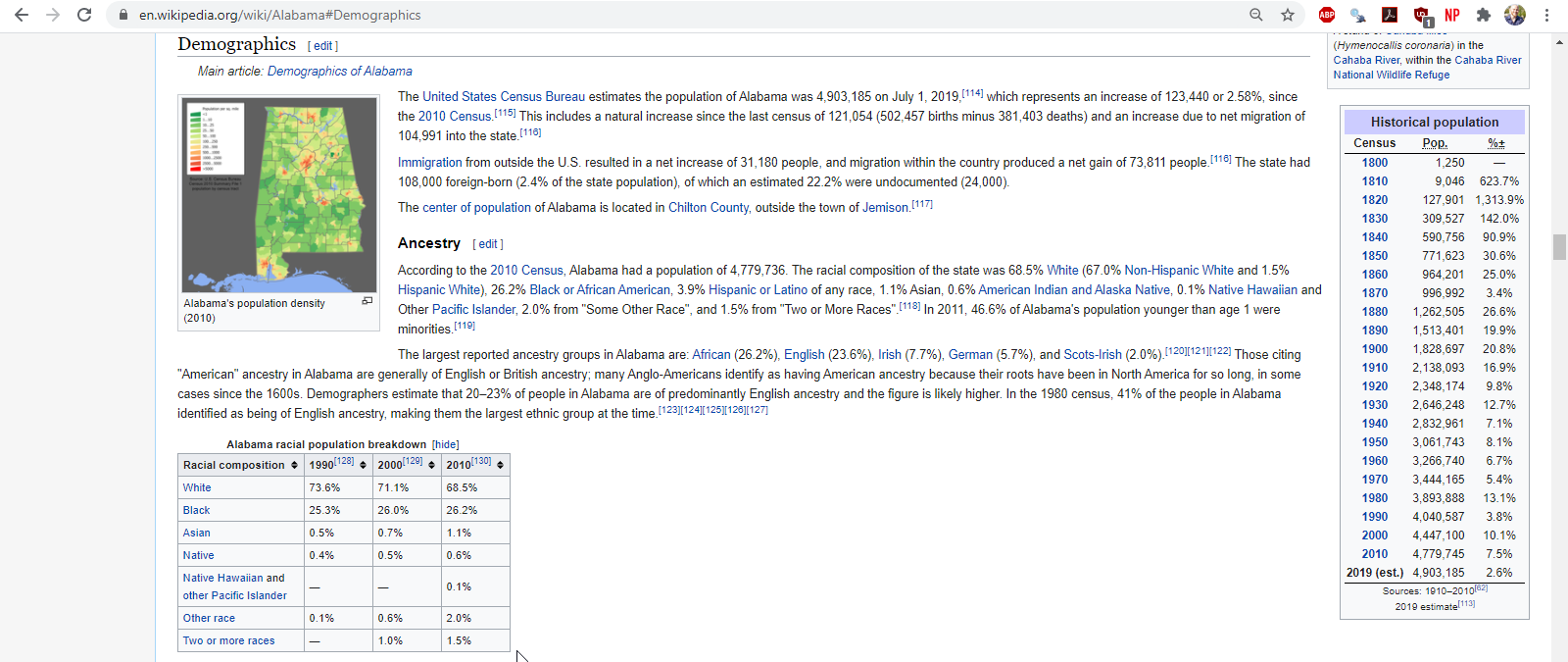
Figure 5.4: part of brainstorming is exploring different websites which may have the data you desire
If we were to go to Georgia, we would notice that the web address is similar to Alabama, but since Georgia is also a country, the web address specifies that you are currently on the webpage for the state rather than the country. This effectively rules out editing the web address to iterate over each state.
If we broaden our search to ‘US States’, we find a Wikipedia page with a list of each state. Each state has a hyperlink which takes us to the state’s webpage with the demographic information we desire. Remember: hyperlinks are our friend! If they exist, we can scrape them, iterating over the web addresses to get data from each state. Let’s use what we just learned to attain the web addresses for each state. We’ll start with the web address containing a list of every state.
wiki_url <- "https://www.wikipedia.org"
states_url <- str_c(wiki_url, '/wiki/U.S._state#States_of_the_United_States')
Let’s use the page source to find where the hyperlinks exist in the HTML code. To do this, I am going to search for the phrase ‘The 50 U.S. states, in alphabetical order, along with each state’s flag’ in the page source since the list of states is just below this phrase.
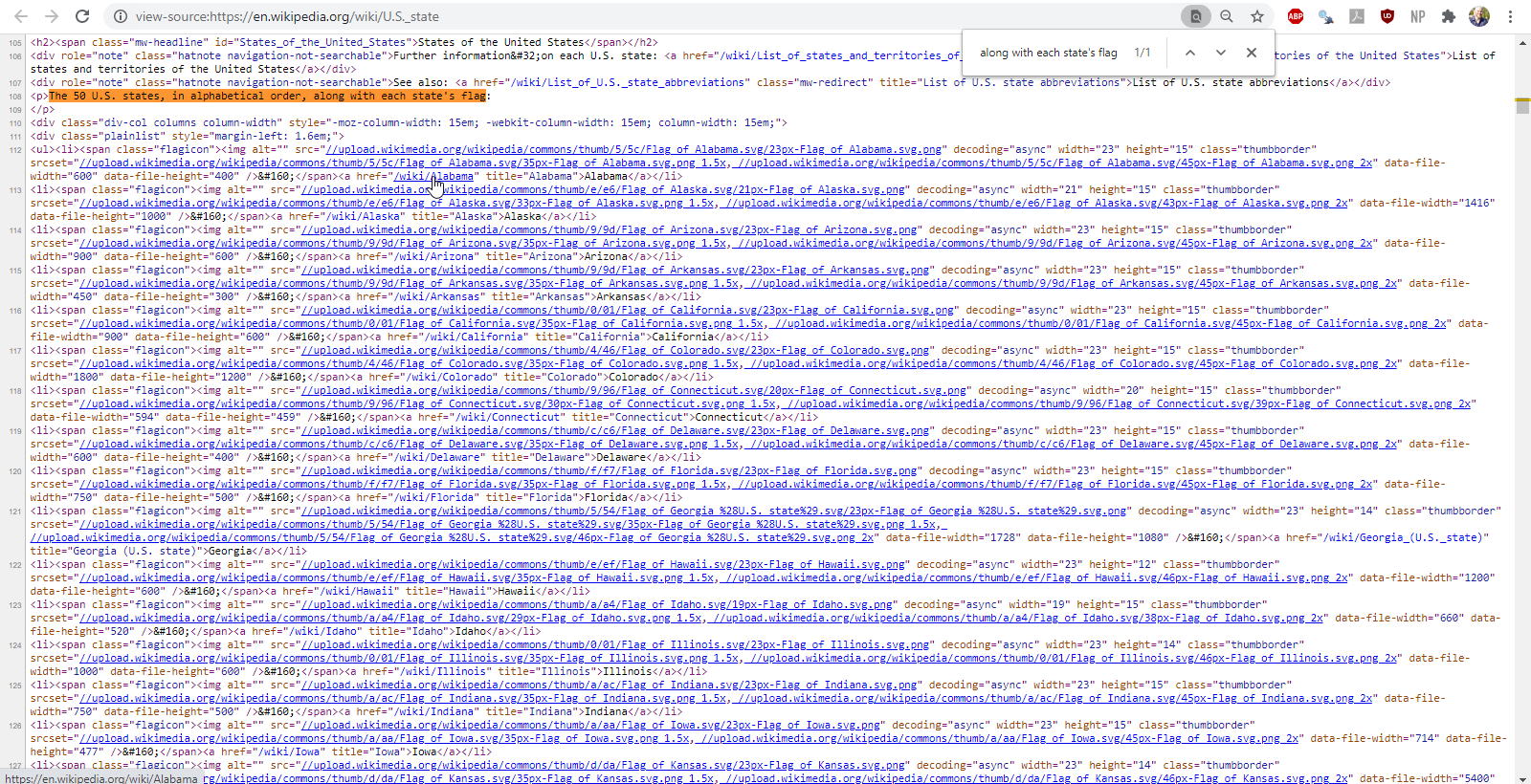
Figure 5.5: finding the element containing the list of states with their cooresponding web addresses using the page source
We find that the list of states, among other information, exists in an element tagged div with the attribute class set to an attribute value of plainlist. Within this node, the list of states exists in an element tagged ul and each state exists in an element tagged li. Within each state, the web address corresponding to that state’s individual Wikipedia article is given in the href attribute to an element tagged a. Let’s use this information to extract the web addresses corresponding to each state. We may also want to extract the state name which is the content of the element tagged a.
node_w_states <- states_url %>%
  read_html() %>%
  html_nodes(xpath = "//div[@class='plainlist']") %>%
  html_nodes('ul') %>%
  html_nodes('li') %>%
  html_nodes('a')

ind_states <- tibble(state = node_w_states %>%
                       html_text(),
                     url = node_w_states %>%
                       html_attr(., 'href') %>%
                       str_c(wiki_url, .))
ind_states
Let’s consider how we would scrape the racial demographics. Use either the selector gadget or the page source to identify where the desired table exists in the HTML code.
ind_states$url[1] %>%
  read_html() %>%
  html_nodes(., xpath = "//table[@class='wikitable sortable collapsible']") %>%
  html_table() %>%
  as.data.frame()
In the next chapter, we will learn the tools to scrape the racial demographics for each state using the vector of web addresses we attained through this process as well as cleaning up these data according to tidy principles.
Any feedback for this section? Click here