3.1 Core Tidyverse
At the heart of Tidyverse are a few packages: dplyr, tidyr, stringr, and forcats. Each package serves a powerful purpose. tidyr helps you create tidy data, while dplyr is used for data manipulation. Think of tidyr as the crowbar or saw in your toolbox, allowing you to bend and shape your data into tidy shape. dplyr, on the other hand, is more like the screwdriver, hammer, or level, allowing you to fix pesky issues with the data. stringr and forcats are useful when working with strings and factors (categorical variables that have a fixed and known set of possible values).
While we will make the effort to teach tidyr and dplyr separately within their own subsections, we recognize that these packages are ultimately created to be used together. Since we may need to make use of functions across packages, we will explicitly state the origin each function by package::function().
3.1.1 tidyr
Let’s take a look at the game by game player rushing and receiving statistics that we scraped using the principles outlined in the previous chapter. To do this, we will first use stringr::str_c(), a function we’ve seen a few times now, to create a web addresses corresponding to Pro Football Reference page for all of the 2020 NFL teams.
pfr_url <- "https://www.pro-football-reference.com"
team_urls <- pfr_url %>%
  # get team abbreviations for all NFL teams and isolate Denver
  get_teams(.) %>%
  # create URLs for all 2020 NFL teams
  stringr::str_c(pfr_url, ., '2020.htm')
as_tibble(team_urls)
Pipes (%>%) make your code much more readable and avoid unnecessary assignments. While not required in many cases, I use a period to indicate where the result to the left of the pipe belongs in the argument to the right of the pipe.
Now that we have the web addresses for every 2020 NFL team, let’s isolate the 2020 Denver Broncos and scrape their players’ aggregated rushing and receiving statistics. We will use dplyr::glimpse() to see the data types and a few values for each column in the data set.
den_stats <- team_urls %>%
  # isolate the 2020 Denver Bronco's URL
  .[10] %>%
  # get team statistics for 2020 Denver Broncos
  get_team_stats()
dplyr::glimpse(den_stats)
Rows: 23
Columns: 28
$ team <chr> "den", "den", "den", "den", "den", "den", "den"~
$ no <chr> "25", "30", "3", "28", "13", "9", "4", "32", "1~
$ player <chr> "Melvin Gordon", "Phillip Lindsay", "Drew Lock"~
$ age <chr> "27", "26", "24", "24", "21", "27", "24", "24",~
$ pos <chr> "RB", "rb", "QB", "", "", "", "", "", "", "", "~
$ games_g <chr> "15", "11", "13", "16", "13", "3", "3", "5", "1~
$ games_gs <chr> "10", "8", "13", "0", "4", "1", "1", "0", "0", ~
$ rushing_att <chr> "215", "118", "44", "35", "9", "6", "5", "4", "~
$ rushing_yds <chr> "986", "502", "160", "170", "40", "28", "-5", "~
$ rushing_td <chr> "9", "1", "3", "0", "0", "0", "0", "0", "0", "0~
$ rushing_lng <chr> "65", "55", "16", "23", "15", "9", "-1", "8", "~
$ rushing_y_a <chr> "4.6", "4.3", "3.6", "4.9", "4.4", "4.7", "-1.0~
$ rushing_y_g <chr> "65.7", "45.6", "12.3", "10.6", "3.1", "9.3", "~
$ rushing_a_g <chr> "14.3", "10.7", "3.4", "2.2", "0.7", "2.0", "1.~
$ rushing_fmb <chr> "4", "0", "8", "0", "2", "0", "1", "0", "2", "0~
$ receiving_tgt <chr> "44", "14", "", "13", "56", "", "", "1", "6", "~
$ receiving_rec <chr> "32", "7", "", "12", "30", "", "", "1", "3", ""~
$ receiving_yds <chr> "158", "28", "", "81", "381", "", "", "5", "26"~
$ receiving_y_r <chr> "4.9", "4.0", "", "6.8", "12.7", "", "", "5.0",~
$ receiving_td <chr> "1", "0", "", "0", "3", "", "", "0", "0", "", "~
$ receiving_lng <chr> "20", "11", "", "28", "49", "", "", "5", "10", ~
$ receiving_r_g <chr> "2.1", "0.6", "", "0.8", "2.3", "", "", "0.2", ~
$ receiving_y_g <chr> "10.5", "2.5", "", "5.1", "29.3", "", "", "1.0"~
$ receiving_ctch_percent <chr> "72.7%", "50.0%", "", "92.3%", "53.6%", "", "",~
$ receiving_y_tgt <chr> "3.6", "2.0", "", "6.2", "6.8", "", "", "5.0", ~
$ yds_touch <chr> "247", "125", "44", "47", "39", "6", "5", "5", ~
$ yds_y_tch <chr> "4.6", "4.2", "3.6", "5.3", "10.8", "4.7", "-1.~
$ yds_y_scm <chr> "1144", "530", "160", "251", "421", "28", "-5",~There are a few things to note after looking at the data, but let’s first consider if these data are tidy. To answer this question, we need more context. If we wished to predict a player’s position based on his statistics, then each player is an observation and his statistics are variables. In this case, these data are tidy in their current wide form, when each player has information in only one row. If we are interested in comparing players across the recorded statistical categories, then an observation would no longer be a player but a player’s statistical category. In this case, these data are tidy in long form, when each player has information in multiple rows. No matter the context, tidyr makes it easy convert your data from wide form to long form with tidyr::pivot_longer() and from long form to wide form with tidyr::pivot_wider().
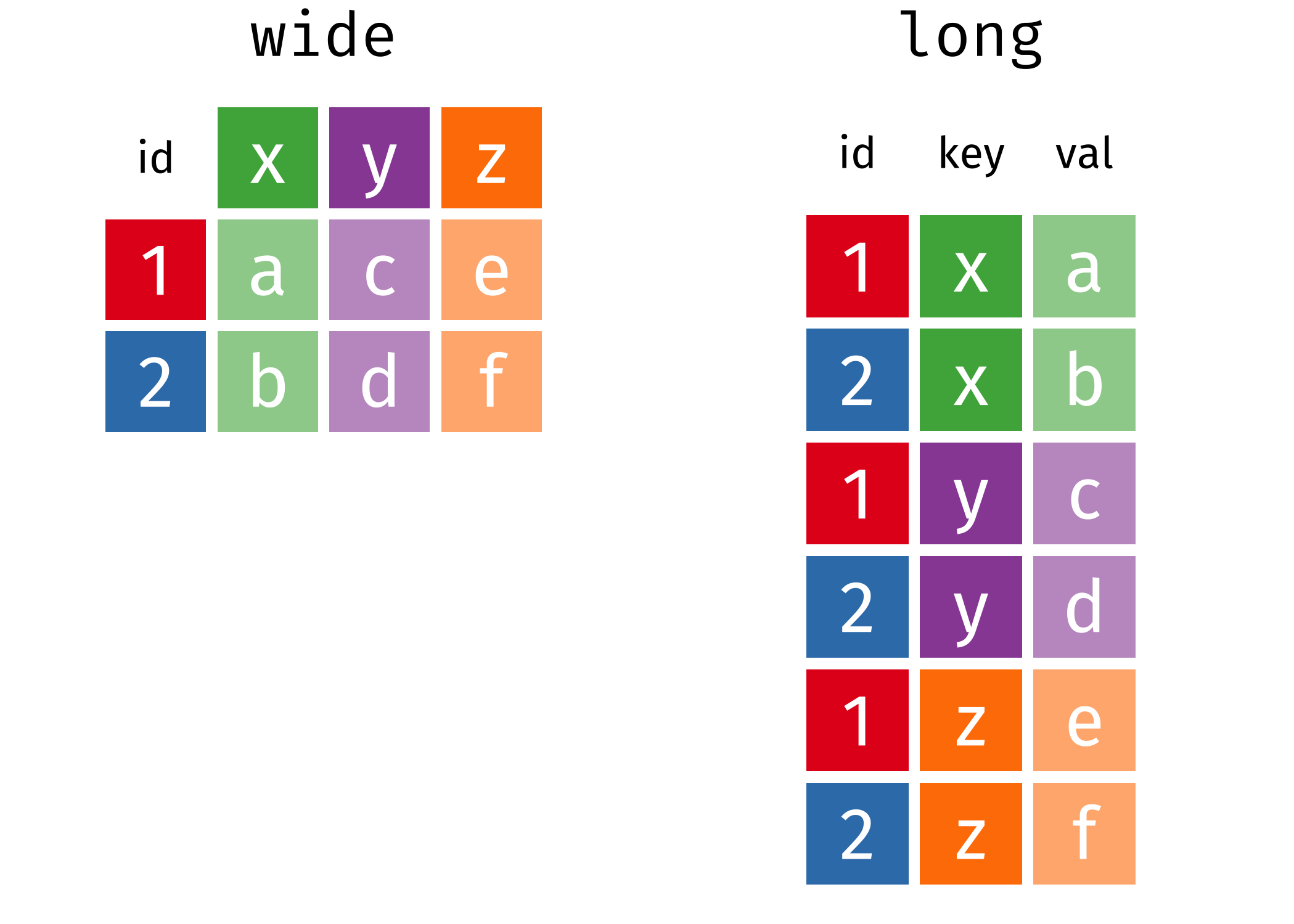
Figure 3.2: visualizing the transformation from wide data to long data, and vice versa
Let’s consider how we can use tidyr::pivot_longer() to tidy these data in preparation for comparing players across their statistical categories. In each row, we should expect to have (1) the player’s name, age, and position, (2) the statistical category, and (3) the value of the statistical category. Imagine taking every other column and pushing them into the rows, duplicating the information above as needed. To do this in R, we will use the dplyr functions dplyr::vars() which allows us to select which variables to push into the rows and dplyr::starts_with() which allows us to pick only variables whose names start with some string. These are two handy functions to know. Further, we will use tidyr::seperate to split the statistical categories into a more general category (i.e. rushing, receiving, etc) and a statistic (i.e. yards per rushing attempt, catch percentage, etc).
den_stats_long <- den_stats %>%
  # push columns into the rows, renaming the names and values columns
  pivot_longer(., cols = c(starts_with('games_'), starts_with('rushing_'),
                           starts_with('receiving_'), starts_with('yds_')),
               names_to = 'stat_category', values_to = 'value') %>%
  # seperate the stat category into a category column and a stat column
  separate(., col = 'stat_category', into = c('category', 'stat'), sep = '_', extra = 'merge')
den_stats_long
If we are in a situation when we are given a data set in long form, but we need it in wide form, we can use tidyr::pivot_wider.
den_stats_wide <- den_stats_long %>%
  pivot_wider(., names_from = c('category', 'stat'), values_from = 'value')
den_stats_wide
After converting back to wide form, the result is the same as the original data set.
3.1.2 dplyr
We’ve addressed how to change the shape of your data using tidyr. Now, we will transition into dplyr where we will outline some of the many functions that can prove helpful in preparing your data for plotting or modeling. Before we jump into various functions, let’s outline the issues with our data set which have not been addressed. The best way to get a sense of the issues is to look at the data.
tibble [23 x 28] (S3: tbl_df/tbl/data.frame)
 $ team                  : chr [1:23] "den" "den" "den" "den" ...
 $ no                    : chr [1:23] "25" "30" "3" "28" ...
 $ player                : chr [1:23] "Melvin Gordon" "Phillip Lindsay" "Drew Lock" "Royce Freeman" ...
 $ age                   : chr [1:23] "27" "26" "24" "24" ...
 $ pos                   : chr [1:23] "RB" "rb" "QB" "" ...
 $ games_g               : chr [1:23] "15" "11" "13" "16" ...
 $ games_gs              : chr [1:23] "10" "8" "13" "0" ...
 $ rushing_att           : chr [1:23] "215" "118" "44" "35" ...
 $ rushing_yds           : chr [1:23] "986" "502" "160" "170" ...
 $ rushing_td            : chr [1:23] "9" "1" "3" "0" ...
 $ rushing_lng           : chr [1:23] "65" "55" "16" "23" ...
 $ rushing_y_a           : chr [1:23] "4.6" "4.3" "3.6" "4.9" ...
 $ rushing_y_g           : chr [1:23] "65.7" "45.6" "12.3" "10.6" ...
 $ rushing_a_g           : chr [1:23] "14.3" "10.7" "3.4" "2.2" ...
 $ rushing_fmb           : chr [1:23] "4" "0" "8" "0" ...
 $ receiving_tgt         : chr [1:23] "44" "14" "" "13" ...
 $ receiving_rec         : chr [1:23] "32" "7" "" "12" ...
 $ receiving_yds         : chr [1:23] "158" "28" "" "81" ...
 $ receiving_y_r         : chr [1:23] "4.9" "4.0" "" "6.8" ...
 $ receiving_td          : chr [1:23] "1" "0" "" "0" ...
 $ receiving_lng         : chr [1:23] "20" "11" "" "28" ...
 $ receiving_r_g         : chr [1:23] "2.1" "0.6" "" "0.8" ...
 $ receiving_y_g         : chr [1:23] "10.5" "2.5" "" "5.1" ...
 $ receiving_ctch_percent: chr [1:23] "72.7%" "50.0%" "" "92.3%" ...
 $ receiving_y_tgt       : chr [1:23] "3.6" "2.0" "" "6.2" ...
 $ yds_touch             : chr [1:23] "247" "125" "44" "47" ...
 $ yds_y_tch             : chr [1:23] "4.6" "4.2" "3.6" "5.3" ...
 $ yds_y_scm             : chr [1:23] "1144" "530" "160" "251" ...
The first issue with the data set that we should address is the inappropriate data types assigned to each column. Every column is scraped as a character, but the players’ position (pos) should be coded as a factor variable and the players’ statistics should be coded as numeric variables. Before we can change the players’ catch percentage (receiving_ctch_percent) to a numeric variable, we first need to remove the percent sign from the values of the variable.
3.1.2.1 mutate
When we wish to change the values within a column, we can leverage the dplyr::mutate() function. Let’s see how we can use some stringr functions within dplyr::mutate() to clean up some of these columns.
den_stats_wking <- den_stats %>%
  mutate(., age = as.numeric(age),
         pos = pos %>%
           str_to_upper() %>%
           na_if(., '') %>%
           as_factor(),
         receiving_ctch_percent = str_remove_all(receiving_ctch_percent, '%'))
den_stats_wking
Within one mutate() call, we (1) recoded the players’ age as a numeric variable, (2) changed the players’ position to uppercase, replaced empty strings with NA values, and recoded the result as a factor, and (3) removed all percent signs from the catch percent statistic. We still need to change all of the players’ statistics to numeric variable. We could do this similarly to the players’ age, but listing out every variable one by one would be painstakingly inefficient. To complete this task, we can use a common variant of the mutate() function called mutate_at() to change every specified column in a similar manner. We can then use mutate_all() to replace every missing string with an NA value, the proper way to specify a missing value in R.
den_stats_wking <- den_stats_wking %>%
  mutate_at(., vars(starts_with('games_'),
                    starts_with('rushing_'),
                    starts_with('receiving_'),
                    starts_with('yds_')),
            ~as.numeric(.x)) %>%
  mutate_all(., ~na_if(.x, ''))
These variants of mutate() (e.g. mutate_at and mutate_all) are aimed to condense code when the same transformation is applied to many columns. To specify the transformation which will be applied to all of the identified columns, you will need a lambda expression. The lambda expressions start with ~ and are followed by a function specifying the transformation such as as.numeric. One of the arguments of the function will be .x which indicates an arbitrary column. To break down the mutate_at() specified above, we seek to transform all columns starting with games_, rushing_, receiving_, and yds_. Overall, there are 23 columns we will be transforming with this single mutate function. The lambda expression ~as.numeric(.x) specifies how to transform each of these 23 columns. That is, for a given column called .x, change .x to be a numeric column. For more information on these variants, also known as scoped verbs (e.g. _if, _at, _all), type ?mutate_if into the console. Several functions we will discuss throughout this chapter also can be used with one of these scoped verbs.
3.1.2.2 slice and filter
Notice, at the bottom of the data set there are two rows which summarize the table. We do not need these rows since they do not outline the performance of an individual player. Keeping these rows would violate the principle of tidy data. There are two approaches we can take to remedy this issue. First, we could consider removing the last two rows of the data set or keeping all rows except for the last two. When we would like to remove or keep rows of a data set using the index of the row, we can leverage the slice() function. To illustrate how to do this, we will use a new helper function n() which returns the number of rows in the referenced data set.
# option 1: remove the last two rows of the data set
den_stats_wking %>%
  slice(., -(n()-1), -n())
# or
den_stats_wking %>%
  slice(., -c(n()-1, n()))

# option 2: keep all rows except for the last two
den_stats_wking %>%
  slice(., 1:(n()-2))
While this certainly solves the issue for this particular data set, it is not a robust solution. If we hope to apply this same logic for other NFL teams, we need to recognize that this solution relies on there only being two total columns which take up the last two rows of the data set. A more robust solution would be to keep only rows consisting of a player not named "Team Total" or "Opp Total". If we want to choose rows based on specific criteria, then we can utilize filter() to choose rows based on specific criteria.
den_stats_wking <- den_stats_wking %>%
  filter(., !(player %in% c('Team Total', 'Opp Total')))
den_stats_wking
3.1.2.3 select
Suppose we’re interested in only rushing and receiving statistics for each of the players.. In this case, we may wish to keep columns containing information on the players and the players’ rushing and receiving statistics. If we want to keep certain columns based on the column names, then we can utilize the select() function. A verbose (but acceptable) solution would be to specify each column we want to keep. To demonstrate, I will keep only information pertaining to the player (e.g. jersey number, name, age, and position).
Since there are several variables for rushing and receiving statistics, we may not want to specify every column name we want to keep. Instead, we can use scoped verbs and helper functions, similar to mutate().
3.1.2.4 group_by
Designed to be used with other functions, group_by groups rows of data set by an attribute. Suppose we’re interested in positions rather than players. In this case, we would like to group players in common positions. When we invoke the group_by function, we are creating a tibble which looks a lot like the original but indicates which rows belong to which group.
[1] "grouped_df" "tbl_df"     "tbl"        "data.frame"
[1] "pos"
Any functions invoked on grouped data will be conducted on the specified groups, rather than the data set as a whole. For example, suppose we’re interested in determining the player with the most receptions by potion. We could utilize the helper slice_max() which will return the row with the largest value for the specified attribute. If we forgot to group the data set by position, then we would return the player with the most receptions, clearly a wide receiver.
If we group by position before invoking slice_max then we would return the players with the most receptions at each of the listed positions. When operating on grouped data, it is important to ungroup when we no longer want operations to be conducted on the groups.
If grouping data confuses you, don’t worry! You are not alone. When using the group_by function, I like to imagine partitioning rows into literal groups and then asking myself what I would like to do with each of the groups. In this case, imagine the coach held a meeting on the field. To start the meeting, he asks all of his running backs (RB) to stand in the home end zone, his wide receivers to stand in the away end zone, and his tight ends (TE) to stand at the home sidelines. All of the other players (with unknown positions) are asked to stand at the away sidelines. In this sense, the coach has created four groups where each group consists of same positioned players. Now, the coach walks to each group individually and asks for the player with the most receptions to follow him. At the end of the day, each group sends one player, so the result is four players.
The group_by function is the coach asking his players to organize themselves on the field, and the slice_max function is asking the player with the largest number of receptions to follow him. Since the slice_max follows the group_by function, the coach for a player from each group.
3.1.2.5 summarize
The summarize function allows us to calculate summary statistics for specified columns. When paired with group_by, the summarize function allows us to calculate summary statistics for each of the groups. For example, suppose I wanted to calculate the average rushing and receiving yards, as well as standard deviations, for each of non-missing positions except for punter. Similar to the mutate, we can specify how we what we want the new columns to be called and how we want to define them.
den_stats_wking %>%
  filter(., pos !='P', !is.na(pos)) %>%
  group_by(., pos) %>%
  summarize(., mean_rushing_yds = mean(rushing_yds),
            sd_rushing_yds = sd(rushing_yds),
            mean_receiving_yds = mean(receiving_yds),
            sd_receiving_yds = sd(receiving_yds))