2.2 Creating an R Markdown Document

The easiest way to create an R Markdown document is to leverage RStudio by navigating to File > New File > R Markdown. You will be asked to populate a few basic options including the Title, the Author, and the Default Output Format. For now, feel free to name your R Markdown document My R Markdown Demo with your name as the author. Keep the default format as HTML. After clicking OK, you will be provided with a default in RStudio’s text editing window. This is where you will create your document.

If you wish to create a PDF using R Markdown, you will need a version of TeX on your computer, a typesetting system. For users who have never interacted with Tex, we recommend installing the tinytex package by running install.packages(‘tinytex’) and then running tinytex::install_tinytex(). After this, you should be able to create a PDF document with R Markdown.

2.2.1 Basic Components

There are three basic components to an R Markdown document: the YAML header, Markdown code, and R code chunks. We will explore each of these components one by one.

2.2.1.1 YAML Header

The YAML header exists at the very top of the R Markdown document. Following my own steps from above, the YAML header to my default R Markdown document looks like:

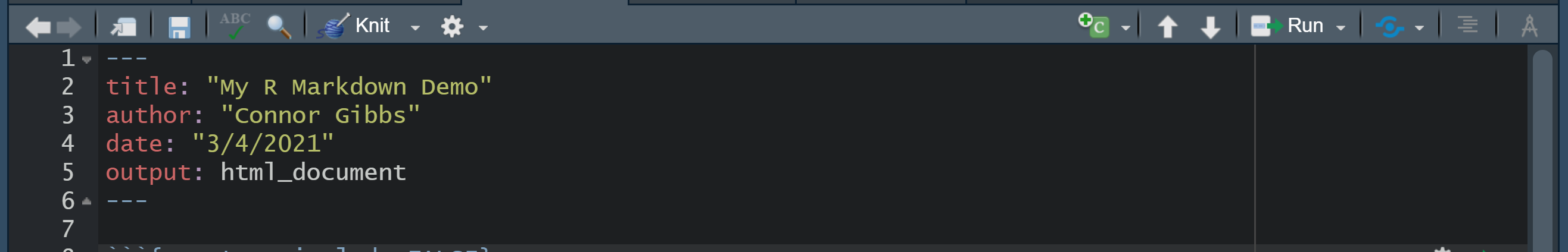
Figure 2.2: example of a YAML header for the default R Markdown template

By default, the YAML header must contain a title, author, date, and output type. Once the YAML header has been specified, you can now knit your document as the specified output type by clicking the Knit icon.

Figure 2.3: icon used to compile and format your R Markdown document

Alternatively, you can create the knitted document programmatically with rmarkdown::render(). Type ?rmarkdown::render into your console for more details. Go ahead and knit your document, and take a look at the default document that is generated. The following two components are included in the default document.

2.2.1.2 R Code Chunks

Code chunks are segments of code throughout your document that will be evaluated sequentially upon knitting. Any output stemming from your code will be included in the final document. An example of an R ‘chunk’ is included below:

```{r}
x <- c(1, 2, 3, 4)
```

All R code chunks are defined in this way; although, you may choose to specify chunk options in the {} of the chunk header. Chunk options allow you to customize how output of a given chunk is portrayed. Any R code can be included within the fences of three back ticks.

While incredibly useful for large blocks of code, code chunks can be an overkill for a small line of code. At times, you may wish to evaluate some R code inline, perhaps to take the sum of x. You can do this by

2.2.1.3 Markdown Code

As we mentioned, markdown is essentially a language used to format a document. When creating your reports in R Markdown, all of your headers, sub-headers, paragraphs, lists, etc. will be included as Markdown code. Thankfully, most of this looks like standard English with a few minor adjustments. Anything that is not your YAML header or contained within an R code chunk (more in a second) is inherently markdown code. We will revist this topic in future chapters when we discuss fine tuning your R Markdown document.